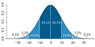
Standard error

For a value that is sampled with an unbiased normally distributed error, the above depicts the proportion of samples that would fall between 0, 1, 2, and 3 standard deviations above and below the actual value.

The standard error, sometimes abbreviated as [math]\displaystyle{ SE }[/math], is the standard deviation of the sampling distribution of a statistic. The term may also be used for an estimate (good guess) of that standard deviation taken from a sample of the whole group.

The average of some part of a group (called a sample) is the usual way to estimate the average for the whole group. It is often too hard or too costly to measure the whole group. But if a different sample is measured, it will have an average that is a little bit different from the first sample. The standard error of the mean is a way to know how close the average of the sample is to the average of the whole group. It is a way of knowing how sure one can be about the average from the sample.

In real measurements, the true value of the standard deviation of the mean for the whole group is usually not known. So the term standard error is often used to mean a close guess to the true number for the whole group. The more measurements there are in a sample, the closer the guess will be to the true number for the whole group.

How to find standard error of the mean

One way to find the standard error of the mean is to have lots of samples. First, the average for each sample is found. Then the average and standard deviation of those sample averages is found. The standard deviation for all the sample averages is the standard error of the mean. This can be a lot of work. Sometimes it is too difficult or costly to have lots of samples.

Another way to find the standard error of the mean is to use an equation that needs only one sample. Standard error of the mean is usually estimated by the standard deviation for a sample from the whole group (sample standard deviation), divided by the square root of the sample size:

[math]\displaystyle{ SE_\bar{x}\ = \frac{s}{\sqrt{n}} }[/math]

where

s is the sample standard deviation (i.e., the sample-based estimate of the standard deviation of the population), and

n is the number of measurements in the sample.

In general, the larger the sample, the closer the estimated standard error of the mean is to the actual standard error of the mean. As a rule of thumb, there should be at least six measurements in a sample. Then the standard error of the mean for the sample will be within 5% of the actual standard error of the mean (that is, if the whole group were measured).

Corrections for some cases

There is another equation to use if the number of measurements is for 5% or more of the whole group:

There are special equations to use if a sample has less than 20 measurements.

Sometimes, a sample may come from one place even though the whole group may be spread out, while other times, a sample may be made in a short time period when the whole group covers a longer time. In which case, the numbers in the sample are not independent, and special equations are used to try to correct for this.

Usefulness

A practical result: One can become more sure of an average value by having more measurements in a sample. Then the standard error of the mean will be smaller because the standard deviation is divided by a bigger number. However, to make the uncertainty (standard error of the mean) in an average value half as big, the sample size (n) needs to be four times bigger. This is because the standard deviation is divided by the square root of the sample size. To make the uncertainty one-tenth as big, the sample size (n) needs to be one hundred times bigger.

Standard errors are easy to calculate and commonly used because:

• If the standard error of several individual quantities is known, then the standard error of some function of the quantities can be easily calculated in many cases;
• Where the probability distribution of the value is known, it can be used to calculate a good approximation to an exact confidence interval;
• Where the probability distribution is not known, other equations can be used to estimate a confidence interval;
• As the sample size gets very large, the principle of the central limit theorem shows that the numbers in the sample are very much like the numbers in the whole group (they follow a normal distribution).

Relative standard error

The relative standard error (RSE) is the standard error divided by the average. This number is smaller than one. Multiplying it by 100% gives it as a percentage of the average. This helps to show whether the uncertainty is important or not.

For example, consider two surveys of household income that both result in a sample average of $50,000. If one survey has a standard error of $10,000 and the other has a standard error of $5,000, then the relative standard errors are 20% and 10%, respectively. The survey with the lower relative standard error is better, because it has a more precise measurement (the uncertainty is smaller).

In fact, people who need to know average values often decide how small the uncertainty should be—before they decide to use the information. For example, the U.S. National Center for Health Statistics does not report an average if the relative standard error exceeds 30%. NCHS also requires at least 30 observations for an estimate to be reported.

Example

Example of a redfish (also known as red drum, Sciaenops ocellatus) used in the example.

For example, there are many redfish in the water of the Gulf of Mexico. To find out how much a 42 cm long redfish weighs on average, it is not possible to measure all of the redfish that are 42 cm long. Instead, it is possible to measure some of them. The fish that are actually measured are called a sample. The table shows weights for two samples of redfish, all 42 cm long. The average (mean) weight of the first sample is 0.741 kg. The average (mean) weight of the second sample is 0.735 kg—a little bit different from the first sample. Each of these averages is a little bit different from the average that would come from measuring every 42 cm long redfish (which is not possible anyway).

The uncertainty in the mean can be used to know how close the average of the samples are to the average that would come from measuring the whole group. The uncertainty in the mean is estimated as the standard deviation for the sample, divided by the square root of the number of samples minus one. The table shows that the uncertainties in the means for the two samples are very close to each other. Also, the relative uncertainty is the uncertainty in the mean divided by the mean, times 100%. The relative uncertainty in this example is 2.38% and 2.50% for the two samples.

Knowing the uncertainty in the mean, one can know how close the sample average is to the average that would come from measuring the whole group. The average for the whole group is between a) the average for the sample plus the uncertainty in the mean, and b) the average for the sample minus the uncertainty in the mean. In this example, the average weight for all of the 42 cm long redfish in the Gulf of Mexico is expected to be 0.723–0.759 kg based on the first sample, and 0.717–0.753 based on the second sample.

Standard Error Media

• 

  Expected error in the mean of A for a sample of n data points with sample bias coefficient ρ. The unbiased standard error plots as the ρ = 0 diagonal line with log-log slope −¹⁄₂.

Related pages

• Errors and residuals in statistics

References

- ↑ "List of Probability and Statistics Symbols". Math Vault. 2020-04-26. Retrieved 2020-09-12.
- ↑ Everitt B.S. 2003. The Cambridge Dictionary of Statistics, CUP. ISBN 0-521-81099-X
- ↑ Altman, Douglas G; Bland, J Martin (2005-10-15). "Standard deviations and standard errors". BMJ : British Medical Journal. 331 (7521): 903. doi:10.1136/bmj.331.7521.903. ISSN 0959-8138. PMC 1255808. PMID 16223828.
- ↑ Gurland, John; Tripathi, Ram C. (1971). "A simple approximation for unbiased estimation of the standard deviation". American Statistician. American Statistical Association. 25 (4): 30–32. doi:10.2307/2682923. JSTOR 2682923.
- ↑ Isserlis, L. (1918). "On the value of a mean as calculated from a sample". Journal of the Royal Statistical Society. Blackwell Publishing. 81 (1): 75–81. doi:10.2307/2340569. JSTOR 2340569. (Equation 1)
- ↑ Sokal and Rohlf 1981. Biometry: principles and practice of statistics in biological research, 2nd ed. p53 ISBN 0716712547
- ↑ James R. Bence 1995. Analysis of short time series: correcting for autocorrelation. Ecology 76(2): 628–639.